June 2020

Any entity or system that we call 'living' will eventually die. This holds at any scale, from cellular level to ecosystems, and even our socio-economic, financial and technological domains.
To understand why, it is best to look at a such a system as an infrastructure for a specific saturation process. Large organisms/systems are actually huge ensembles of interacting (and saturating) sub-processes, but here we just consider the 'top-level' saturation process. (At a high, technical abstraction level, this is always the saturation-process of entropy production, and the system is some local maximum of this, but you can read about this in our other publications).

This saturation process can mathematically be illustrated with so-called 'limit cycles'. Many biological processes have been described as such, when they show 'periodic' or 'cyclical' behavior (such as cellular processes, heart-dynamics, etc). A limit cycle is like the optimal cyclical or periodical movement of the state of a system. Because of the surrounding noise of other related dynamics, this optimal or 'perfect' path is not perfectly followed, but this path can be seen as an 'attractor' for the state of a system. However, the attracting reach of such a limit-cycle is limited. A large 'perturbation' (a shock) can kick the system out of orbit, and the system will find the nearest other attractor (if it exists).
This kind of limit cycle is called 'stable' because as long as the systems stays in its 'bandwidth' it will be attracted towards it. There are also 'unstable' limit cycles, which actually drive systems away from it. So, in huge systems with lots of (hierarchical) structures of stable and unstable limit-cycles for its subsystems, one can see the intricate complexity of its dynamics, and the subtlety of 'robust' systems.

Most of the scientific research on these systems involves the determination of some limit cycle for some process. However, since these systems are ultimately a saturation of something, the limit cycle itself will change as well. This is only visible on a larger timescale.
In between these 2 scales, there can be other factors that change these limit cycles. Think of our economy, for example, and infrastructural changes. One can then look at the industrial revolution and the IT-revolution as significant (economic and financial and social and technical) infrastructural changes, that alter the existing limit cycles that attract the economic state to some optimum, for that moment. Several other subsystems (i.e. their limit-cycles) need to realign to these changes as well, but will do so in different speeds, and non-linearly. In abrupt changes, this may cause turbulence.

So, we must distinguish between 2 kinds of dynamics: the dynamics of the state of the system around some limit cycle, and the dynamic of the limit cycle itself. (Actually, in lots of systems, the dynamics of a limit cycle can be driven by a hierachically 'higher' limit cycle, etc etc. like a fractal).

Bifurcations

It is even possible for a stable limit-cycle to become unstable. This is called a 'bifurcation', a qualitative change (which can be quantified btw). Obviously, this may have severe implications for the system, but it can be beneficial for the hosting system. For example, every day lots of your bodily cells die, and make place for new cells (apoptosis) But for now, let's not look at 'beneficiality', but just at understanding the dynamics.

So, in short, a dynamic system (organism/economy/etc) can only exist as long as its state-space has a stable limit-cycle, around which the state of the system can revolve. As the entropy-production of this system saturates, this limit-cycle becomes unstable (a bifurcation) or reaches such a state. And during the stable phase, a living system can still perturbate out of its stability region (by sickness, poisening, an accident, etc).

To illustrate this, we have created an animation of the saturation process of a system, as a changing limit cycle. It is not the system itself, but the 'space' in which the system can exist, and a specific region in this space where the system is stable.

However, a single stable limit cycle has an infitely large basin of attraction, so the system can't really get out of its basin of attraction. Therefore we have added two unstable limit cycles (one outer, one inner). This yields a 'bandwidth' of attraction around the center limit-cycle. We have colored this region green (it will appear at some point in the animation).
The animation just shows a 'perfect' lifecycle of a system: it starts by being 'born' (a closed circle emerges: this is the stable limit-cycle), and then it develops a bandwidth of stability (between the 2 green concentric circles). Again, during this phase, a large perturbation can kick the system out of the green basin of attraction of this attractor, and it will collapse (by the surrounding unstable limit cycles).
After reaching some maximum, the bandwidth around the circle decreases (saturation progresses): the stable limit-cycle has bifurcated into an unstable one, and the system collapses.
Obviously, in reaching the end, even smaller perturbations may already kick the system out of stability, before reaching the saturation point.

Asymptotic versus bifurcating saturation

Let's go one step further, and distinguish between asymptotic saturation, and bifurcating saturation.
(Actually, instead of asymptotic we are talking about logistic saturation, but the last part of a logistic process looks asymptotic: it approaches but never reaches a limit-value.) As stated, in reaching the bifurcation to an unstable limit cycle, the bandwidth of stability may be so small, that even a slight shock might already kick the system of out stability.
Maybe, some systems actually never really saturate, but reach this saturation-level slower and slower, ad infinitum, and the environment shows such a distribution of perturbations that the probability that the system is kicked out of the basin of attraction by this becomes so high, that at a saturation-level of, say, 95%, no system will survive these perturbations anymore. (This replaces the 'need' for an actual bifurcation.) We have created an animation for this 'asymptotic bifurcation' as well. The green bandwidth decreases, but will never reach an actual end-point. It shows the development of the so-called phase-portrait of the system.

However, this thesis does allow for tail-events that keep some systems alive disproportionally long (relative to the hosting system, or surrounding population). Many ordinary populations of organisms show nice normal distributions of age, so this suggest that an actual bifurcation level is often reached (otherwise we expect to see tail-events that would really skew a Gaussian age-distribution).
In the actual case of a proportionally 'strong' perturbation distribution (coming from a noisy environment, or internal dynamics, etc), this difference matters less, however.

A 3D-version of a bifurcating limit cycle

Steps towards a diagnostic toolset of systemic health

There are many types of systems, but in understanding and analysing them, we need to distinguish between:

• state-dynamics around the limit-cycle versus limit-cycle-dynamics (both influence the robustnest of the system)

Next to that, in some analytical usecases, we may need to assess whether:

• the environmental perturbation-distribution outweighs the difference between an asymptotic and a bifurcating saturation scenario (because maybe in some cases where it is hard to determine the saturation-type, it doesn't even matter)

Kate Raworth's doughnut

In trying to construct useful new and more inclusive 'economic' policy-frameworks, the economist Kate Raworth has proposed the 'doughnut model', where the relevant human and natural domains are represented, and are allocated a threshold of 'systemic health'. They are visualized as a doughnut, where metric aspects of these domains can be within this doughnut-threshold (healthy) or show too little or too much momentum and fall outside the doughnut (which is bad for systemic health).
The animations show a doughnut-shape as well. Although these models are domain-agnostic, at the human scale they share the conceptual notion with Raworth's doughnut: try to keep stuff within the doughnut for 'stability'. It is all about managing systemic integrity, but we still need a mapping from the technical aspects describe here, to the anthropocenic policy-frameworks and methodogies that Raworth addresses.

A note

Please remember these models are extremely simplified and illustrative versions of reality. In reality, such attractors are high-dimensional and much more intricate ('strange attractors').

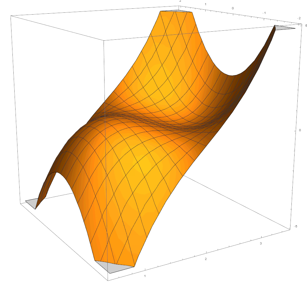
For those interested, the differential equations used to generate these phase portraits are (in polar coordinates):
- bifurcating:
\[ \dot{r} = (r-1)(r-2)(r-3)+(r-2) \tau^2, \dot{\theta}=1 \]
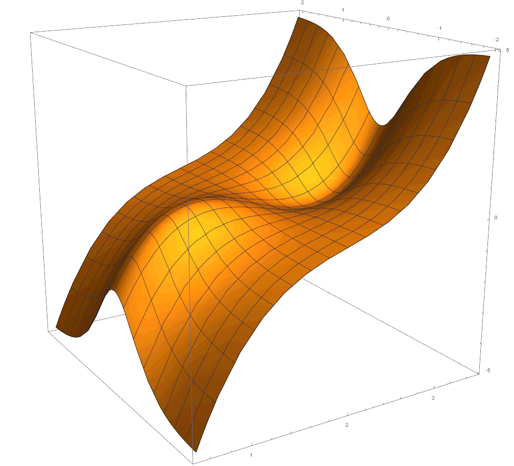
- logistic\asymptotic:
\[ \dot{r} = (r-1)(r-2)(r-3)+(r-2) (1+\cfrac{1}{1-2e^{\tau ^2}}), \dot{\theta}=1 \]

For convenience, the plots of state variable \( r \) against system parameter \( \tau \) are shown below.